Co-benefits of carbon neutrality in enhancing and stabilizing solar and wind energy

Anthropogenic climate warming has led to more frequent climate extremes^1,2,3,4 and pollution episodes^5,6,7, which pose a serious threat to economy, ecological environment and human health^8,9. To limit global warming to well below 2 °C above pre-industrial levels, global carbon neutrality must be achieved by the second half of the twenty-first century¹⁰. Achieving global carbon neutrality requires >50% reductions in anthropogenic carbon dioxide (CO₂) emission by 2030^11,12, driven by an accelerated transition to renewable energy.

Solar photovoltaic (PV) and wind energy are major drivers of clean energy transition; however, unlike nuclear or geothermal, their power outputs are sensitive to meteorological conditions^13,14,15,16. Sunlight captured by a PV module is influenced by solar altitude angle and sky condition¹⁵. For example, clouds and aerosols can decrease sunlight reaching the ground by scattering and absorbing solar radiation, leading to smaller solar power yield¹⁷. In addition, high ambient temperature also reduces the conversion efficiency of solar panels¹⁸. The wind power yield is dominated by wind speed at the hub height (100–150 m) of wind turbines¹⁹. Generally, neither smaller nor larger wind speed weathers are optimal to wind energy generation, because wind turbines (for example, Sinovel SL3000) typically start generating power at 3 m s⁻¹, but need to shut down at 25 m s⁻¹ for safety concerns²⁰.

Therefore, climate change projections provide key information for long-term planning and investment of solar and wind energy infrastructures. Many studies have assessed global or regional solar PV and wind energy, typically under the high-emission scenarios of the IPCC’s Representative Concentration Pathways (RCPs) and Shared Socioeconomic Pathways (SSPs)^{20,21,22,23,24,25,26}. However, very few studies have examined solar PV and wind energy under the low-warming scenarios (notable exceptions being refs. ^24,27 on scenarios reaching net zero after 2080). Such a lack of analysis in the past was probably due to the general perception that low-emission pathways are difficult to achieve given existing climate policies and a lack of coordinated global climate model runs. The COVID-19 pandemic recovery may have provided a vital opportunity to fast-track climate change mitigation²⁸, and indeed more than 120 nations have recently pledged to reach net zero carbon emissions by the mid-twenty-first century (2040–2060)^29,30,31.

Recent studies show that deep CO₂ emission cuts (along with aerosol decline from co-emission sources) can have major impacts on future climate, such as mitigated climate extremes^12,32,33,34. Therefore, a systematic assessment of both solar PV and wind energy under a carbon-neutral climate is needed to understand how they change from now and how they differ from other high-warming scenarios studies. Here, we present the first study, to our best knowledge, of quantifying solar PV and wind energy under deep mitigation scenarios, by leveraging a newly available large multi-model ensemble projection generated at the wake of the COVID-19 green recovery. To explore the potential impacts of COVID-19 lockdowns in 2020 and post-pandemic green recovery, a new model intercomparison project (CovidMIP) was conducted by six Earth system model (ESM) modelling groups³⁵. Assuming a fast renewable transition during the post-pandemic recovery, two emission scenarios reaching global carbon neutrality by 2050 and 2060 are designed in CovidMIP, which are contrasted with a well-studied weak mitigation scenario of SSP2-4.5, without reaching net zero before 2100. Our assessment of global solar PV and wind energy under the deep mitigation pathways, using a bias-corrected large ensemble of simulations with particular attention on the temporal intermittency of energy availability, will provide valuable support for decision-making in renewable energy investments across regions and sources.

Solar PV is an important renewable supply to meet the ambitious climate change mitigation target. Here, we assess the solar PV potential (PV_POT) under different climate change scenarios (Fig. 1 and Supplementary Fig. 1). The ensemble mean simulation projects that the solar PV_POT increases by ~4% in eastern China and ~3% in the eastern United States and western Europe during 2040–2049 under SSP2-4.5 relative to the historical period (Fig. 1a). However, a large decline by approximately 4% is found over India, and also slight decrease but with high inter-model agreement over southern South America, central Asia, Australia, Africa and the western United States. Although this ensemble consists of four models, the spatial pattern of changes is consistent with other multi-model studies on SSP2-4.5 or higher-emission scenarios using the models from the Coupled Model Intercomparison Project Phase 6 (CMIP6)^36,37.

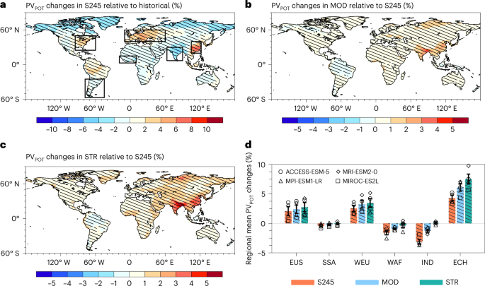
a, The relative changes of annual mean solar PV_POT (%) during 2040–2049 under SSP2-4.5 (S245) relative to the historical period. b,c, The relative changes of annual mean solar PV_POT during 2040–2049 under the moderate (MOD; b) and strong (STR; c) mitigation scenarios relative to S245. Hatched regions have changes with high inter-model agreement defined as at least three of the four models agreeing on the sign of changes. d, Regional mean relative changes of annual solar PV_POT during 2040–2049 under S245 (red bars), MOD (blue bars) and STR (green bars) scenarios, all relative to the historical period. The markers are individual model values and the bars (black error bars) represent the mean values (one standard deviation) of four climate models. The hatched red (blue and green) bars have changes with high inter-model agreement during 2040–2049 under S245 (MOD and STR) relative to the historical period (S245). The six sub-regions with large emissions are marked with black boxes: eastern United States (EUS), southern South America (SSA), western Europe (WEU), western Africa (WAF), India (IND) and eastern China (ECH) (Supplementary Table 2).

Full size image

The solar PV_POT in the mid-twenty-first century can be strongly influenced by global carbon-neutral policies (Fig. 1b,c). In eastern China, the increase in solar PV_POT during 2040–2049 in SSP2-4.5 relative to the historical period is projected to be further enhanced by another 2% and 3% in the moderate (MOD) and strong (STR) scenarios, respectively. In India and western Africa, the projected decrease in solar PV_POT during 2040–2049 in SSP2-4.5 can be offset back to the historical level in the STR scenario (IND and WAF in Fig. 1d). In the eastern United States and western Europe, there is only weak enhancement of solar PV_POT during 2040–2049 in the carbon-neutral scenarios compared with SSP2-4.5, but with high inter-model agreement (EUS and WEU in Fig. 1d). These results highlight a major co-benefit of carbon-neutral policies by enhancing solar PV_POT in the mid-twenty-first century over global land regions except for the Amazon, which is also clear when considering the resource quality of solar energy (Extended Data Fig. 1 showing absolute change).

The solar PV_POT is sensitive to multiple meteorological factors, including surface downwelling shortwave radiation, temperature and wind speed (Methods). By fixing certain meteorological variables and varying others, we further decompose their individual contributions to solar PV_POT changes under different scenarios (Fig. 2). Overall, solar PV_POT changes under SSP2-4.5 relative to the historical period are mainly dominated by surface downwelling shortwave radiation (I) and temperature (T; Fig. 2a,b), with limited contributions from wind speed (W; Fig. 2c). For regions with increased solar PV_POT, including the eastern United States, western Europe and eastern China, although the increase of surface downwelling shortwave radiation is the main driver (Extended Data Fig. 2b), there are relatively small negative contributions from temperature because a warmer solar panel is less effective in converting solar energy into electricity (Extended Data Fig. 2a). For regions with decreased solar PV_POT (Fig. 1a), contributions from temperature (increasing; Extended Data Fig. 2a) and surface downwelling shortwave radiation (decreasing; Extended Data Fig. 2b) are in the same direction and generally comparable in southern South America, India and western Africa, but a dominant contribution from the increasing temperature is found in the western United States.

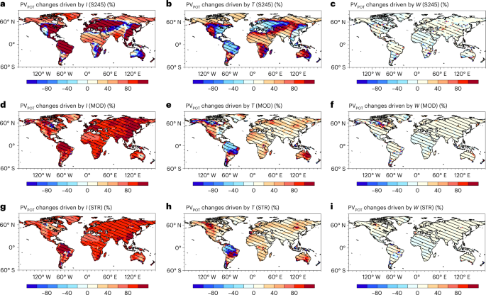
a–c, The relative contributions of surface downwelling shortwave radiation (I; a), temperature (T; b) and wind speed (W; c) to solar PV_POT (%) changes during 2040–2049 under S245 relative to the historical period. d–f, The relative contributions of I (d), T (e) and W (f) to solar PV_POT changes during 2040–2049 under MOD relative to S245. g–i, The relative contributions of I (g), T (h) and W (i) to solar PV_POT changes during 2040–2049 under STR relative to S245. Hatched regions have changes with high inter-model agreement defined as at least three of the four models agreeing on the sign of changes.

Full size image

In contrast to the governing factors for solar PV_POT changes under SSP2-4.5, surface downwelling shortwave radiation (Fig. 2d,g), not temperature (Fig. 2e,h), contributes most of the enhanced solar PV_POT in Asia (especially in eastern China and India) under carbon-neutral scenarios (MOD and STR) relative to the baseline scenario. The surface downwelling shortwave radiation increased notably in Asia under the carbon-neutral scenarios (Extended Data Fig. 2d,f), which improves solar energy harvesting. It is well known that surface downwelling shortwave radiation is primarily influenced by clouds and aerosol loadings^38,39,40,41. We note that aerosol optical depth shows a large decline by 30–40% in eastern China and India during 2040–2049 under two carbon-neutral scenarios relative to SSP2-4.5 (Supplementary Fig. 2b,d). In contrast, a slight increase in cloud fraction is found over the same regions (Supplementary Fig. 2a,c). Therefore, the aerosol optical depth decrease due to sharp aerosol emission reductions in the carbon-neutral scenarios is the dominant factor driving the large increase in solar PV_POT in Asia. This co-benefit of air quality improvement in China in enhancing solar PV was similarly reported recently⁴², but focusing on the historical trend during 1995–2014.

We select a typical wind turbine of Sinovel SL3000 as an example to assess the wind energy under different climate scenarios (Fig. 3 and Supplementary Fig. 3). Relative to the historical period, annual mean wind power (WP) increases by >25% in the tropics and the southern subtropics but decreases by >10% in the northern mid-high latitudes during 2040–2049 under SSP2-4.5 (Fig. 3a). Such a strong interhemispheric asymmetry response of WP to future warming was also identified by another recent study²¹, which attributed the decreased WP in the northern mid-high latitudes to polar amplification and the increased WP in the tropics and the southern subtropics to enhanced land–sea thermal gradients. Regionally, WP shows a large decrease (~8%) in the eastern United States but a moderate increase (3–6%) in western Africa, southern South America, India, eastern China and southeastern Asia during 2040–2049 under SSP2-4.5 relative to the historical period (red bars in Fig. 3d).

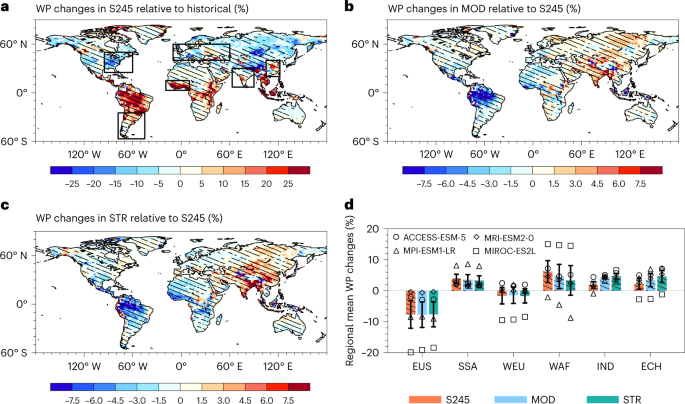
a, The relative changes of annual mean WP (%) during 2040–2049 under S245 relative to the historical period. b,c, The relative changes of annual mean WP during 2040–2049 under MOD (b) and STR (c) relative to S245. Hatched regions have changes with high inter-model agreement defined as at least three of the four models agreeing on the sign of changes. d, Regional mean relative changes of annual WP during 2040–2049 under the S245 (red bars), MOD (blue bars) and STR (green bars) scenarios relative to the historical period. The markers are individual model values and the bars (black error bars) represent the mean values (one standard deviation) of four climate models. The hatched red (blue and green) bars have changes with high inter-model agreement during 2040–2049 under S245 (MOD and STR) relative to the historical period (S245).

Full size image

We further quantify how the projected changes in WP in the mid-twenty-first century can be affected by global carbon-neutral policies (Fig. 3b,c). The main feature of WP changes under deep mitigation scenarios is a west-to-east shift, instead of the north-to-south shift as noted in Fig. 3a. That is, in Asia, especially in eastern China but broadly in South Asia and northern Eurasia, the increase in WP during 2040–2049 relative to the historical period is further enhanced from 2% in SSP2-4.5 to 3% in the moderate carbon-neutral scenario (MOD) and 5% in the strong carbon-neutral scenario (STR). In contrast, the increase in WP in western Africa during 2040–2049 is reduced from 6% in SSP2-4.5 to 3% in the STR scenario (Fig. 3d). Such a major shift of wind energy resources towards Asia in the mid-twenty-first century driven by global carbon-neutral policies can be found more clearly from the absolute changes (Extended Data Fig. 3b,c), which consider the spatial heterogeneity of actual WP output (Supplementary Fig. 4). The changes in wind power density (WPD) also broadly match the spatial pattern of WP response to the carbon-neutral policies, only with slightly smaller magnitude (Extended Data Fig. 4).

WP changes are mainly caused by a shift in different wind speed conditions (Equation (9) in Methods). We further show the frequency changes of different wind speeds under future scenarios (Fig. 4). There are obvious changes for days below the cut-in wind speed (W < 3 m s⁻¹) and within the ramp-up wind speed (3 ≤ W ≤ 11), but limited changes in rated-power wind speed (11 < W ≤ 25). Furthermore, spatial patterns of changes in cut-in and ramp-up wind speed days largely resemble those of WP. For example, more days under the ramp-up wind speed and less days in cut-in wind speed are found in eastern China and India (Fig. 4d,e,g,h), contributing favourably to the enhanced WP during 2040–2049 under the MOD and STR scenarios relative to the baseline scenario. In regions with weakened WP, such as western Africa, the day below cut-in wind speed is increased, but days with ramp-up wind speeds are decreased. Our findings reveal the critical role of shifts between cut-in and ramp-up wind speeds, rather than days with optimal conditions (rated-power wind speed of 11–25 m s⁻¹), in governing future WP changes. Note that the WP results are presented here with an illustrative wind turbine and the results may change quantitatively for other types of turbine with different (ideally lower) cut-in wind speed. Nevertheless, in general, our results suggest the importance of accurately modelling low wind conditions in climate model projections.

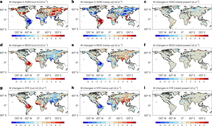
a–c, The frequency changes (d yr⁻¹) of cut-in (W < 3 m s⁻¹; a), ramp-up (3 ≤ W ≤ 11 m s⁻¹; b) and rated-power (11 < W ≤ 25 m s⁻¹; c) wind speed conditions during 2040–2049 under S245 relative to the historical period. d–f, The frequency changes of cut-in (d), ramp-up (e) and rated-power (f) wind speed conditions during 2040–2049 under MOD relative to S245. g–i, The frequency changes of cut-in (g), ramp-up (h) and rated-power (i) wind speed conditions during 2040–2049 under STR relative to S245. Hatched regions have changes with high inter-model agreement defined as at least three of the four models agreeing on the sign of changes.

Full size image

Temporal variability is a key aspect of renewable energy sources, which strongly affects the stability of energy supply, leading to concerns about its large-scale deployment. Therefore, quantifying how the temporal variability of solar PV and wind energy changes in future is crucial for planning complementary energy sources and storage to secure a stable and reliable energy supply.

Using the normalized mean absolute deviation (NMAD), we show the variabilities of solar PV_POT and WP at various time scales in the historical period (Extended Data Fig. 5). The global variabilities of solar PV_POT and WP all decrease from daily to monthly, and then to yearly, scales. This is because the seasonal cycle is stronger than inter-annual variation for meteorological variables. However, solar PV_POT and WP show an opposite spatial pattern in all day-to-day, month-to-month and year-to-year variabilities. From tropical to mid-high latitudes, the variability of solar PV_POT increases (Extended Data Fig. 5a,c,e), while the variability of WP decreases gradually (Extended Data Fig. 5b,d,f). Solar PV_POT mainly depends on sunlight capture and cell temperature. The strong seasonal variation in solar altitude angle in the mid-high latitudes causes large disturbance to local surface downwelling shortwave radiation and temperature, leading to unstable solar power output. But WP is dominated by wind speed at the hub height of wind turbines. In the tropics, the large variability of wind speed due to ocean–atmosphere oscillations results in unstable wind energy output²².

Climate change influences not only annual mean generation of solar PV and wind energy, but also its variabilities at various time scales. We show the changes in day-to-day, month-to-month and year-to-year variabilities of solar PV_POT and WP during 2040–2049 under three future climate change scenarios, all relative to the historical period (Fig. 5). For solar PV_POT, a higher temporal stability of daily and yearly solar PV outputs is found in the eastern United States, southern South America, western Europe and eastern China, which show large decreases during 2040–2049 under SSP2-4.5 (Fig. 5a,e). However, the solar PV_POT in western Africa and India show large increases of day-to-day and month-to-month variabilities but decreases of year-to-year variability during 2040–2049 under SSP2-4.5. For WP, the day-to-day and month-to-month variabilities both increase obviously in the eastern United States and India, indicating a weaker temporal stability of WP during 2040–2049 under SSP2-4.5 (Fig. 5b,d). In contrast, day-to-day and year-to-year variabilities decrease in western Africa and eastern China, suggesting a greater temporal stability of daily and yearly WP during 2040–2049 under SSP2-4.5 (Fig. 5d,f).

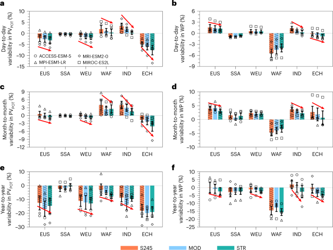
a,c,e, The relative changes in day-to-day (a), month-to-month (c) and year-to-year (e) variability of solar PV_POT during 2040–2049 under S245 (red bars), MOD (blue bars) and STR (green bars) relative to the historical period. b,d,f, The same but for relative changes in day-to-day (b), month-to-month (d) and year-to-year (f) variability of WP. The markers are individual model values and the bars (black error bars) represent the mean values (one standard deviation) of four climate models. The hatched red (blue and green) bars have changes with high inter-model agreement defined as at least three of the four models agreeing on the sign of changes during 2040–2049 under S245 (MOD and STR) relative to the historical period (S245). The six sub-regions are defined in the Fig. 1 caption.

Full size image

Although there are large regional differences in changes of solar PV_POT and WP variabilities during 2040–2049 under SSP2-4.5, we find that the changes of solar PV_POT and WP variabilities due to global carbon-neutral policies (indicated by the red arrows in Fig. 5) are overall consistent in most of sub-regions focused on here. The day-to-day, month-to-month and year-to-year variabilities of solar PV_POT decrease in five sub-regions (except for southern South America) during 2040–2049 under two carbon-neutral scenarios (MOD and STR) relative to SSP2-4.5. Furthermore, the day-to-day, month-to-month and year-to-year variabilities of WP decrease in the eastern United States, western Europe, India and eastern China during 2040–2049 under two carbon-neutral scenarios of MOD and STR relative to SSP2-4.5, with the exceptions in southern South America and western Africa with less changes (Fig. 5b,d,f). These findings indicate that global carbon-neutral policies improve the temporal stability of daily, monthly and yearly WP and solar PV_POT during 2040–2049 in most of global land regions studied here.

Although recent studies have assessed renewable energy resources in response to future climate change^{20,21,22,23,24,25,26,43}, several knowledge gaps remain to be filled for making sound clean energy policies: (1) many previous analyses focused on high-warming scenarios of RCP8.5 or RCP4.5, but the COVID-19 pandemic may have provided a vital opportunity to accelerate the renewable transition in coming decades faster than assumed in previous high-warming scenarios; (2) most studies were limited to regional scale or a certain type of renewable energy, while a global analysis is needed to provide an integrated assessment towards building a comprehensive energy supply system; (3) the variability across various time scales is generally missing in previous regional assessments of renewable energy, despite being known as a major issue strongly affecting the stability and reliability of energy supply; and (4) previous assessments calculated the 100 m wind speed from 10 m wind speed using a constant scaling factor, which thus has probably introduced a large bias in projected wind energy (Supplementary Fig. 5). Leveraging on previous studies, our analysis presents a comprehensive global assessment of both solar PV and wind energy, including annual mean power potential as well as temporal stability at various time scales. Our analysis is based on large multi-model ensemble simulations (2400 model years of daily data) that are bias-corrected using a multivariable approach. We estimate the wind speed at 100 m using a spatially variant scaling factor, which is closer to benchmark. The model projections are run under two deep decarbonization scenarios, reaching global carbon neutrality much earlier than previous scenarios.

Our findings that climate change mitigation would improve the mean solar PV in Europe, India and China are qualitatively consistent with previous assessments comparing other emission scenarios (for example, RCP2.6 versus 6.0 and RCP4.5 versus 8.5)^24,43,44, but with notable magnitude difference. For example, in contrast to decreased solar PV in India at the end of the twenty-first century (2070–2100) under RCP2.6 scenario²⁴, we find that the projected decrease in solar PV will rebound to the historical level by the mid-twenty-first century (2040–2049) in the STR scenario (Fig. 1d). The north-to-south interhemispheric shift of wind energy under SSP2-4.5 relative to the historical period largely agrees with an early study²¹, but our study highlights a notable west-to-east shift of wind energy due to deep decarbonization. Regionally, the large enhancement (>20%) of wind energy in western Africa during 2040–2069 under SSP5-8.5 relative to the historical period⁴⁵ would be weakened to 3% during 2040–2049 in the STR scenario (Fig. 3d). The further enhancement in solar PV and wind energy is mainly attributed sharp reductions in anthropogenic aerosol emissions (Supplementary Fig. 2). Aerosol emissions reduction can improve the solar energy capture (due to larger surface downwelling shortwave and, to a lesser extent, the cooler PV cells) and increase the favourable ramp-up wind speed conditions.

Reaching global carbon neutrality by the mid-twenty-first century is a bold goal for climate change mitigation. More than 120 nations, contributing 70% of global CO₂ emissions, have pledged to reach net zero carbon emissions by the mid-twenty-first century^31,46. Meanwhile, the installation of renewable energy capacity, including solar PV and wind, is accelerating worldwide. It is expected that the global renewable energy capacity will increase by about 75% in the next five years⁴⁷. Although the world is moving in the right direction, much needs to be done to reach net zero carbon emissions by the mid-twenty-first century. A few recommendations can be made based on the analysis here. (1) Coordination of renewable energy capacity building at the international level is required due to large regional differences in renewable energy quality (Extended Data Fig. 6). (2) Planning of complementary energy sources because the projected power potentials’ response to future climate change are different for different types of renewable energy. For example, solar PV increases but wind energy decreases in western Africa due to deep decarbonization (Figs. 1 and 3). (3) Smart design of energy transmission and storage due to the temporal intermittency of renewable energy. Each country should set their own priorities based on underlying climate and climate projection, local resources, expertise and technologies.

Some uncertainties are acknowledged here. First, the wind energy and solar PV_POT are estimated on a daily scale due to model output availability. Here, we compare wind energy and solar PV_POT calculated based on daily and hourly fifth generation European Centre for Medium-Range Weather Forecasts (ERA5) reanalysis during 1995–2014. The daily-based wind energy underestimates hourly-based wind energy by 7.4% on global average due to high frequency fluctuation averaged out at the daily level (Supplementary Fig. 6). On the contrary, the daily-based solar PV_POT shows a positive bias of 6.3% on global average compared with hourly-based solar PV_POT (Supplementary Fig. 7). By fixing two of three hourly variables and varying the third daily variable, we further show that such positive bias of solar PV_POT is mainly dominated by daily surface downwelling shortwave radiation (Supplementary Fig. 8b), with limited contributions from daily temperature and wind speed (Supplementary Fig. 8a,c). Second, the temporal variability within a day is not included, again due to lack of sub-daily model output. The solar PV_POT shows a strong intra-daily variability: zero during the night and peaking in the noontime^48,49. Compared to solar PV_POT, the wind energy is relatively stable in a day. However, observational studies showed that wind energy tended to be unstable in a day under clear-sky rather than all-sky conditions⁵⁰. Third, climate feedback due to constructed wind or solar farms is not considered in the model simulations here. Previous studies show that the installed wind turbines and PV panels would modify land surface properties, such as roughness and albedo, resulting in changes in regional climate^51,52,53.

Despite these limitations, our results are valuable in making sound long-term plans of renewable investments across global regions. The findings that some regions are projected to observe large co-benefits of wind energy and solar PV associated with deep decarbonization could, in turn, support a faster clean energy transition to achieve the carbon-neutrality target, hence completing a favourable human–nature feedback loop. This is in stark contrast with previously reported detrimental feedback loops, for example, where global warming could reduce the potential capacity of bioenergy with carbon capture and storage⁵⁴, damaging the chances of meeting the global carbon-neutrality goal. In order to facilitate the transition into a global economy powered by clean energy, international coordination should be strengthened further, due to the spatial, temporal and technological imbalance of renewable energy resources.

CovidMIP simulation

The multi-model ensemble simulations from CovidMIP were used to investigate changes in solar PV and wind energy potentials in response to carbon-neutral policies. In CovidMIP, the baseline scenario follows the SSP2-4.5, a medium pathway of future greenhouse gas emissions with a global mean warming of about 2 °C in the 2050s and 2.6 °C in 2100⁵⁵. Accounting for anthropogenic emissions decline during the COVID-19 pandemic and the possible fast renewable transition during the post-pandemic recovery, CovidMIP produced two carbon-neutral pathways from 2020 to 2050: a moderate green recovery (MOD) and a strong green recovery (STR)³⁵. These two carbon-neutral scenarios both include a ‘two-year-blip’ period (2020–2021), which is not the focus of our analysis here, followed by the moderate MOD and faster STR scenarios towards reaching global carbon neutrality by 2060 and 2050, respectively.

Six ESMs participated in CovidMIP, four of which, ACCESS-ESM-5, MIROC-ES2L, MPI-ESM1-2-LR and MRI-ESM2-0 (Supplementary Table 1), are used here, because they made available daily output of surface air temperature (T), surface downwelling shortwave radiation (I) and 10 m wind speed (W, calculated by meridional and zonal winds), which are necessary to quantify solar PV and wind energy, especially their day-to-day variability. All four models provided large ensemble simulations (30-member for ACCESS-ESM-5 and MIROC-ES2L, and 10-member for MPI-ESM1-2-LR and MRI-ESM2-0), which allows a robust quantification of projection uncertainty. In addition, the same number of simulations for each model (as in Supplementary Table 1) are selected from the historical experiment (1995–2014) from CMIP6 to evaluate model skill and correct biases, and to provide a base period to quantify future changes of solar PV and wind energy. In this study, we first calculate renewable energy in individual ensemble members, which is then averaged to each model and the multi-model generation.

Bias correction

To evaluate model performance in simulating solar PV and wind energy during the historical period (1995–2014), we obtain daily (averaged from hourly) T, I and W (calculated by meridional and zonal winds) from the ERA5 reanalysis. ERA5 has been evaluated extensively in earlier studies and is found to be one of the best global reanalysis products^56,57, widely used as a benchmark to evaluate and correct model simulations^58,59. An early study showed that the ERA5 reanalysis overestimated global I by 4.05 W m⁻² (~3%) using site-based solar radiation from the Baseline Surface Radiation Network⁵⁷. Here, we further evaluate T and W from the ERA5 reanalysis based on global observations at 3,511 weather stations. Compared with observations, the ERA5 reanalysis well captures global T and W with low normalized mean biases of −0.2% and 3.0%, respectively (Supplementary Fig. 9), much smaller than model–ERA5 discrepancy (Extended Data Fig. 6c,d). To maintain the consistency of spatial resolution among the four ESMs, both reanalysis and model outputs are re-gridded to a median resolution of 2 × 2° using the bilinear interpolation method. To improve the robustness of the model projection, we use the multivariate bias correction technique based on the n-dimensional probability density function transform (MBCn) to simultaneously correct daily T, I and W in historical and future model simulations using the ERA5 reanalysis as the benchmark.

MBCn is a multivariate generalization of quantile delta mapping, which considers the dependence among different variables⁶⁰. In using MBCn, three datasets are included: historical observations (X_obs), historical simulations (X_hist) and projected simulations (X_proj). First, we rotate X_obs, X_hist and X_proj with an N × N uniformly distributed random orthogonal rotation matrix R^[j] at the jth iteration:

Second, the quantile delta mapping method uses the same empirical cumulative distribution function (CDF) for simulations (historical and future) and observation, but it preserves the signal of future changes in climate projections⁶¹. This method is applied to obtain bias-corrected datasets in historical and projected simulations (({hat{X}}_{{{mathrm{hist}}}}^{[j]}) and ({hat{X}}_{{{mathrm{proj}}}}^{[j]})):

where F_hist and F_proj represent the CDFs of ({widetilde{X}}_{{{mathrm{hist}}}}^{[j]}) and ({widetilde{X}}_{{{mathrm{proj}}}}^{[j]}), respectively. ({F}_{{{mathrm{obs}}}}^{-1}) and ({F}_{{{mathrm{hist}}}}^{-1}) represent the inverse CDFs of ({widetilde{X}}_{{{mathrm{obs}}}}^{[j]}) and ({widetilde{X}}_{{{mathrm{hist}}}}^{[j]}), respectively.

Finally, the bias-corrected datasets are rotated back:

For historical or projected simulation correction, we repeat the above three steps until the multivariate distribution of ({X}_{{{mathrm{hist}}}}^{[j+1]}) or ({X}_{{{mathrm{proj}}}}^{[j+1]}) matches that of X_obs.

The MBCn is applied to individual members of each ESM’s simulation, separately.

Calculation of solar PV

Solar PV power yield depends on PV power generation potential (PV_POT) and installed capacity. PV_POT is a dimensionless value, which describes the performance of PV cells relative to the nominal power capacity under actual environmental conditions. Therefore, PV_POT multiplied by the nominal installed watts of PV power capacity is the actual PV power generation. Following previous studies^15,43,62, we used daily T, I and W to calculate PV_POT:

where I represents surface downwelling shortwave radiation and I_STC represents shortwave flux on the PV panel under standard test conditions, defined as a constant of 1,000 W m⁻². P_R is the performance ratio, representing temperature influence on PV efficiency:

where γ is defined as −0.005 °C⁻¹ in monocrystalline silicon solar panels, representing the negative impact on conversion efficiency, and T_STC is the cell temperature under standard test conditions (25 °C). T_cell is the actual cell temperature, which is approximated by T, I and W:

where a1, a2, a3 and a4 are taken as 4.3 °C, 0.943 (unitless), 0.028 °C (W m⁻²)⁻¹ and −1.528 °C (m s⁻¹)⁻¹, respectively. These coefficients represent the influence of meteorological conditions on the cell temperature. The ambient T determines the base temperature of the cell, a strong I increases the cell temperature and W decreases cell temperature. These coefficients are found to be fairly independent on site location and cell technology type⁶³, which have been widely used to predict PV cell temperature^15,43,64.

Calculation of wind energy

WPD (W m⁻²) is a typical measure of wind energy potential⁶⁵, defined as follows:

where ρ represents the air density, which is assumed to be a constant value of 1.213 kg m⁻³ at standard atmospheric conditions, and W_h represents the wind speed at the 100 m hub height.

It is noted that W_h is not available from climate model outputs here. Similar to previous studies^22,23,25, W_h is extrapolated from the 10 m wind speed (W) using the wind power law:

where W_z represents the wind speed at a height z and ({W}_{{z}_{{{mathrm{ref}}}}}) represents the wind speed at a reference height z_ref. The scaling factor of α, representing how quickly the wind decays towards the ground, is often approximated as a constant of 0.143 over land surface in previous studies^22,26,45. As the ERA5 reanalysis provided wind speeds at both 10 m and 100 m, here we estimate α at each location grid (Extended Data Fig. 7) to account for spatial disparity. The higher values of 0.2–0.25 are mainly located in the eastern United States, eastern China, Amazon, India and northern Asia due to large forest coverage, but the lower values of 0.12–0.16 usually occur in flat terrain of desert and steppe. As an improvement to a few previous studies using a constant scaling factor^21,22, the wind speed at 100 m here estimated using a spatially variant scaling factor is closer to the benchmark (Supplementary Fig. 5c versus b). The normalized mean bias decreases from −10.1% to −0.4% on global average. In contrast to the large spatial heterogeneity, the scaling factor only shows a small temporal variability (Supplementary Fig. 10 showing seasonal change as an example), resulting in limited benefits on estimation of 100 m wind speed (Supplementary Fig. 5d versus c; −0.4% improved to −0.3%). Therefore, the spatially variant but temporally invariant scaling factor is adopted here to estimate 100 m wind speed from the 10 m wind speed in the model output.

The actual wind power (WP in KW) is sensitive to wind speed and wind turbine. Here, we adopt a typical wind turbine of Sinovel SL3000 (https://en.wind-turbine-models.com/turbines/41-sinovel-sl3000-113) as an example to describe WP²⁰:

where the turbine starts functioning at 3 m s⁻¹, generating the rated-power of 3,000 KW at 11 m s⁻¹ or above, but needs be shut down at 25 m s⁻¹. Therefore, 3 m s⁻¹ and 25 m s⁻¹ are defined as cut-in and cut-out speeds, respectively. The wind speed of 3 to 11 m s⁻¹ is defined as ramp-up condition and the wind speed of 11 to 25 m s⁻¹ is defined as rated-power condition.

Temporal variability of solar PV and wind energy

For both solar and wind energy, we first calculate the daily value using model outputs, which is then averaged to monthly and annual generation over all locations. It is well known that solar PV and wind energy generation are heavily influenced by weather fluctuation, which yields strong variability at various time scales. Understanding the variability of renewable energy is vital for coordinating compensatory energy sources and storage in order to secure a stable energy supply^66,67.

Here, we use the metric of NMAD to quantify the day-to-day, month-to-month and year-to-year variability of renewable energy. For any given time series (T_i, i = 1,2,…N), the NMAD (%) is defined as the mean absolute deviation divided by the mean:

For day-to-day and month-to-month variability of solar PV and wind energy, we first calculate the corresponding NMAD for each year, and then present the multi-year average of NMAD.

Model evaluation with bias correction

Climate model simulations of solar PV and wind energy resources remain highly uncertain^21,36,45. Here, we evaluate the simulated solar PV and wind energy in the historical period (1995–2014) against ERA5 (Extended Data Fig. 6). The observed solar PV_POT shows a smooth global spatial contrast (Extended Data Fig. 6a). In global arid and semi-arid regions, including the western United States, northern Africa, western Asia and Australia, the solar PV_POT shows higher values of >0.24. However, the solar PV_POT is relatively lower in global monsoon regions, including east Asia, south Asia, central Africa, southeastern North America and the Amazon. Such a spatial pattern can be attributed to more clouds in those monsoon regions and possibly denser vegetation cover, leading to less solar radiation available at the ground level^68,69,70. Compared with reanalysis, the raw output from model simulation overestimates the solar PV_POT by more than 15% in southeastern Asia, the Amazon and western Africa, but underestimates it by approximately 10% in the western United States, northeastern Asia and western Asia (Extended Data Fig. 6c). Using the MBCn technique to jointly correct T, I and W, the calculated solar PV_POT from the model simulation agrees well with the observation, with a relative bias of less than 1% over all land grids (Extended Data Fig. 6e).

In contrast to the solar PV_POT, the observed annual mean WPD shows very large spatial heterogeneity (Extended Data Fig. 6b). The large values of >160 W m⁻² are mainly located in the central United States, Europe, midwestern Australia, northern Africa and northern Asia. The annual mean WPD of 60–100 W m⁻² is found in eastern China, India and southern Africa. However, the annual mean WPD is smaller than 20 W m⁻² in the tropics, including the Amazon, central Africa and southeastern Asia, where there are light winds due to a small horizontal temperature gradient and large surface friction over vegetated lands. Compared with observation, the raw ensemble mean simulation shows very large biases across the world, with a mean relative bias of 49.4% over global lands (Extended Data Fig. 6d). Regionally, simulated annual mean WPD is overestimated by more than 100% in the western United States, northern Africa, India, Australia and most of Asia, but underestimated by 50–70% in Europe, the Amazon and central Africa. After the MBCn bias correction, the simulated annual mean WPD is close to observation at both global and regional scales (Extended Data Fig. 6f). The global spatial relative bias decreases from 49.4% to −7.5%. In most regions of the world (other than Greenland and southern Australia), the relative bias is smaller than 15%.

The evaluations demonstrate the need of bias correction to improve the fidelity of model simulations. Here, the same bias correction is applied to the ensemble future projection in CovidMIP to investigate the future changes in solar PV and wind energy. This type of multivariant bias correction for climate variables has been done for many climate impact studies^71,72,73, but not in previous renewable energy resources analysis. Compared with an early assessment based on traditional bias-corrected climate data²⁴, our study uses the MBCn method, which considers the dependence across climate variables, and represents an advance from the widely used single-variable bias correction.